A place for discussions and planning for the Nuclear Structure Spring 2024 course
Some resources about Bayesian statistics for context for the first homework:
Bayesian Statistics
-
FRIB Summer School materials:
-
Video on Bayesian statistics by Frederi, Pablo, and Nori
More resources:
-
Starting programing:
- Becoming a Git Guru. More on Github. Even more on Git Hub
- Here goes a repository with a first guided example on how to run jupyter notebooks in code spaces. In the README file there is a link to a video recorded by Kyle and me on how to go through it too.
-
Nuclear Physics:
- Slides of a presentation on nuclear theory. It has some good slides about the liquid drop model!
- Introduction paper
Here goes a repository with a first Jupyter notebook for solving for the wave functions on a WoodsSaxon potential by varying the energy.
You can use it to explore resonances but also modify it to find bound states and how they evolve when the bound energy approaches the threshold!
We could also use it to host cool codes you folks make in this course ![]()
Hey friends!
Some folks have asked what they should use for the “errors” associated with the masses for the first project, since the table only had the values of N, Z, and BE/A (without errors). I have a short, long, and very long answers to that:
-
Short: Make the least square fit and estimate the error size from that. This is related to the “s” factor Witek has on slide 15 of lecture “3. Binding”.
-
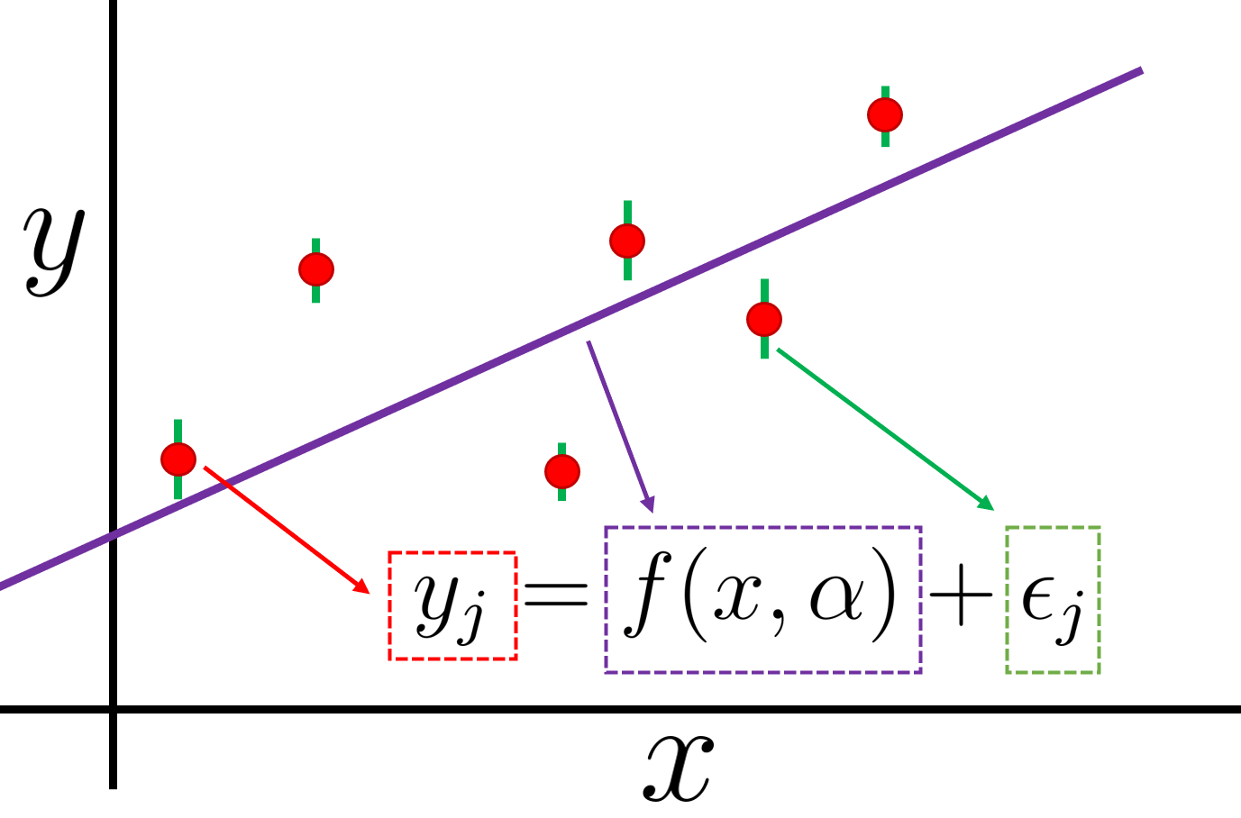
Long: When you are fitting or calibrating a physical model with data, you need to come up with a statistical model for how the physical model and the observed data relate to each other. The simplest (most of the time not-very-correct) assumption you can make is that your model is perfect (captures all the physics), and any deviation between theory and experiment comes from random independent Gaussian errors and these are the experimental errors themselves. If we have given you the associated BE/A errors, you could have used those, but the problem is that they will never explain the deviations between your model and the observations (they are way too tiny!). This situation resembles this picture:
in where the deviations between data (red points) and theoretical model (purple line) can’t be explained by the tiny experimental errors alone (in green). The subscript “j” goes from 1 to 6 for the six data point. This equation represents a statistical model, we take into account our physical model f (with parameters \alpha ) together with our model on how the data “fluctuated” around our physical model.
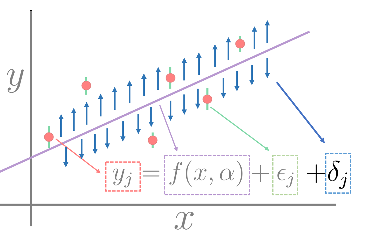
A way to improve this statistical model is to add a term that accounts for “model error”, and is there to explain deficiencies (missing physics) in our physical model. It is harder to make a pictorial representation of this, but my best try is:
It is kind of a thing that pushes data points away from the central model, and it can be either up or down and has (in our simplest assumption) a more or less constant expected size. It is a hard thing to estimate because if you knew it exactly, your model would be perfect. You can, nevertheless, estimate it using statistical approaches and treat it as if it were random, that is what most people do on the first approximation. This is the error size that you are expected to use on your statistical analysis of the homework, and you need to estimate in some way. The simplest (but not the only) way to estimate it is to make a least squares fit, compute the root mean squared error of your model (sum the residuals squared, take average, take square root), and that would give you a sense of its scale (this is related to the “s” factor that Witek has in the slides). If this scale comes to be 0.3 MeV (just as an example) that does not mean that the LDM makes an error of exactly 0.3 MeV on every sample, rather than its errors are distributed (we hope…) as a Gaussian with standard deviation ~ 0.3 MeV.
Long Long: Watch the videos on Bayesian statistics and the slides we described above. Check also how we created our statistical model in Sec 4 of this paper, in which we were actually calculating binding energies and decided to neglect the experimental errors in favor of the model ones. Check out Figure 4 of that paper for another visual interpretation
For Homework 2, for the MHO frequency, it says “plus sign holds for neutrons and the minus sign holds for protons”. I’m confused because I thought the energy levels for protons were shifted up by the coulomb barrier, not down.