The easiest way to ask my question is by describing the scenario. It seems like a fun problem, but I’m not sure where to start.
For the description, let’s consider a set of data with 100,000 events. Assume there is a multiplicity distribution (Gaussian is fine) describing the number of particles in each event. Event one may have 10 particles, event two may have 4 particles, etc.
For each event we wish to make a calculation (call this an “event observable”) by summing all the particle data in said event. Per event, each particle in the event has an unknown parameter associated to it that, if optimized, would make the calculation “better”.
Here comes the catch: Each parameter for each particle is initialized to 1, and you have no knowledge of what the final distribution of your parameters should be. Further, you don’t know what the final distribution of your event observables should be.
There are two metrics to work with to determine how well your parameters are optimized.
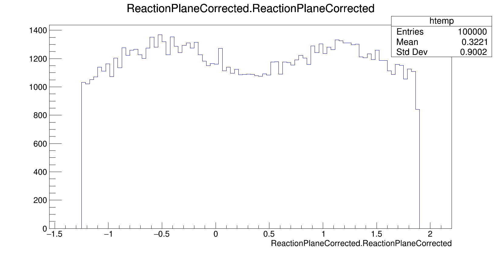
After creating a distribution of event observables, you can pass this distribution into a black box that will apply a series of corrections. If your parameters are optimized, the output distribution from the black box will look isotropic. The less optimized your parameters are, the less isotropic your black box output will be. Assume that deviations from the optimal parameter values monotonically change the isotropicity of the black box distribution.
After creating a distribution of event observables, the distribution is randomly shuffled and split into two equal size distributions. Take the absolute difference between the two random samples; the more Gaussian the difference is, the better your parameters are.
Given this scenario, what technique would be best in determining the optimal parameter distribution?
Tagging @pablo while I think about it! Also will tag @Edgard since he likes these kind of problems.
@Sam, do you have any pictures of the distributions pre/post optimization? I know you tried a simple optimization with -1,0,1 (if I remember correctly)
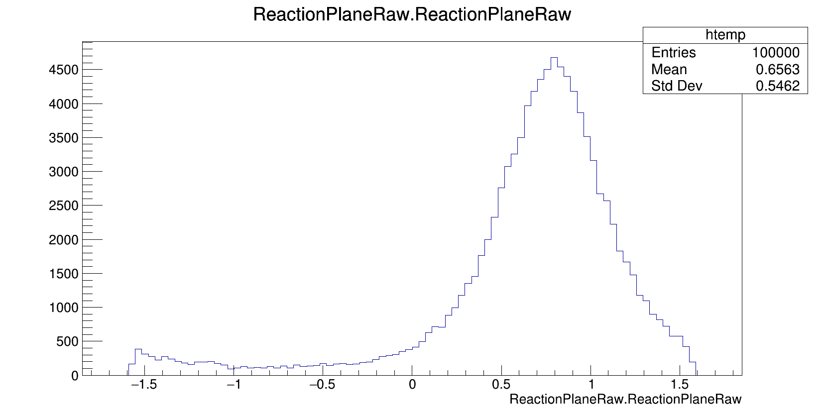
Just to clarify, this plot is the distribution of event observables with a weighting scheme of -1, 0, 1. The weights are assigned conditionally based on other observable information (rapidity in this case).
And do the weights have some physical interpretation? I can always shuffle data around to get a uniform distribution, but I presume that’s not enough lol
I wish. The weighting scheme is based on particle rapidity. If a particle is in a range of a reactions midrapidity region, the weight is set to 0. If the rapidity is larger than the midrapidity region, the weight is set to 1.
btw I’m performing this analysis in the lab frame. The -1 and 1 come from reflection symmetry in the center of mass frame, so the weights I have right now don’t really make sense.
Seems interesting, but I’m still uncertain on what is it that you want to calculate. I will ask a few clarifying questions to try to parse what is it that you’re looking to do:
You have a collection of events. Each event can be modeled as an independent realization of the same experiment, is that correct?
Each event is characterized by having a [discrete] number of “particles” that contribute to it. The number of particles of each event is not fixed, but it can be modeled as following some probability distribution. Is this still correct?
For each event, you are extracting a quantity which you call an “event observable” that you are recording. What is this quantity, mathematically? you said it is a sum of “all the particle data” in an event, could you clarify?
There is a blackbox that applies “corrections” to the observables —> The output of the blackbox has an “isotropic” distribution. What does Isotropic mean? uniform, diagonal covariance Gaussian? What does the blackbox do? If the blackbox is invertible, then you already know what your target distribution is by the implicit function theorem.
The distribution of event observables is such that two randomly drawn observables from the distribution are (ideally?) Gaussian distributed? If so, that actually really constrains the family of functions that your distribution can be (see characteristic functions, convolutions, etc.) Is this the case?
Each particle in each event has three quantities associated to it: \theta, \phi, and a weight w. For an event with N particles, the event observable I’m calculating is defined as \frac{1}{N}\arctan\bigg(\sum_{i}^{N} \frac{w_{i}sin(\phi_{i})sin(\theta_{i})}{w_{i}cos(\phi_{i})sin(\theta_{i})}\bigg).
The output from the black box should be a Gaussian distribution. The box achieves this by recentering the original distribution about the mean and fitting the distribution with a Fourier expansion to find a shift for every event observable.
The difference between two randomly drawn observables should be Gaussian. Thanks for the suggestions, I’ll start reading.
For point 3.
Looking at your equation. Isn’t that just the average phi_i? Or am I missing something? Is there a typo on the equation?
For point number 5:
When you look at the definition of the characteristic function (which can be seen as a glorified fourier transform) of a probability distribution, notice that the characteristic function of P(x) and that of P(-x) are complex conjugates of one another. Moreover, they also must be reversed in the ““fourier”” parameter. Since we are assuming that you are drawing two independent copies (say, X and Y) of a distribution, then the characteristic function of the random variable Z=X-Y is the squared modulus of the amplitude of the characteristic function for X. Since this last one you tell me is Gaussian, then it is straightforward to see that the characteristic function of X should look like:
exp(i*f(t)-1/2Var(X)*t^2), where f(t) is an odd function of t.
Therefore it might be worth considering using characteristic functions (fourier transforms of prob densities) rather than the densities themselves.
Thank you for pointing that out, the sum should be inside of the arctan function.
I’m pretty unfamiliar with characteristic functions, so I’ll come back to this post with more questions after I get through some reading. Thanks for pointing me in a direction!!